Lattice quantum mechanics in 1d

This post has been migrated from my old blog, the math-physics learning seminar.

For some reason I’ve been interested in lattice QFT recently, especially lattice gauge theory (note to self: a miniproject for the Christmas break is to understand the paper by Kogut and Susskind http://prd.aps.org/abstract/PRD/v11/i2/p395_1). As a warm-up, I thought I would try understanding plain-old 1D QM on the lattice, and writing some code to see if I got results that are at all reasonable.

The Setup: We will take as our space of states (\mathscr{H} = L^2([0,1])) and hamiltonian

$$

H = -\frac{d^2}{dx^2} + V(x).

$$

for some real function (V(x)) defined on ([0,1]).

Now fix some large positive integer (N). Let (\epsilon = 1/N). We will consider the subspace (\mathscr{H}_N) of (\mathscr{H}) spanned by those functions that are constant on the subintervals (i\epsilon, (i+1)\epsilon)). Such a function is defined (a.e.) by the (N) values it takes on these intervals, so we may identify (\mathscr{H}_N \cong \mathbb{C}^N) as vector spaces. Let us denote elements of (\mathscr{H}_N) by (\psi_i) for (i = 0, \ldots, N-1). Thinking of these as the values of a function (\psi(x)) at (x = i\epsilon), we see that the inner product on (\mathscr{H}_N) is given by

$$

(\phi, \psi) = \int_0^1 \bar{\phi}(x) \psi(x) dx = \sum_{i=0}^{N-1} \bar{\phi}_i \psi(i)

$$

So we see that with these identifications, (\mathscr{H}_N) is just (\mathbb{C}^N) with the usual hermitian inner product.

Now, we can approximate (d/dx) with the forward and backward difference operators

\begin{align}

(D_+ \psi)_i &= \frac{\psi_{i+1} - \psi_i}{\epsilon} \

(D_-\psi)_i &= \frac{\psi_i - \psi_{i-1}}{\epsilon}

\end{align}

Note: throughout I will assume periodic boundary conditions to make life easy. In this case we have (\psi_{i+N} = \psi_i).

Now consider

\begin{align}

(D_+\phi, \psi) &= \epsilon^{-1} \sum_i \left( \bar{\phi}_{i+1}\psi_i - \bar{\phi}_i \psi_i \right) \

&= \epsilon^{-1} \sum_i \left( \bar{\phi}i \psi{i-1} - \bar{\phi}_i \psi_i \right) \

&= -(\phi, D_-\psi).

\end{align}

Thus we have (D_+^\ast = -D_-). Similarly, (D_-^\ast = -D_+). Then the operator (D = (D_+ + D_-)/2) approximates (d/dx) and satisfies (D^\ast = -D) (as it should!), and the discrete Laplacian (D^2) is self-adjoint.

Finally, we can form the discrete hamiltonian (H_N) by taking (H_N = -D^2 + \hat{V}), where (\hat{V}) is the operator (\psi_i \mapsto V(x_i) \psi_i), where (x_i = i\epsilon).

Note: typically one further imposes Dirichlet or Neumann boundary conditions. This corresponds to projecting to a smaller subspace of (\mathscr{H}_N).

I wrote some Sage code to test this. With (V(x) = 0), and (N = 500), here is one of the lowest-energy states:

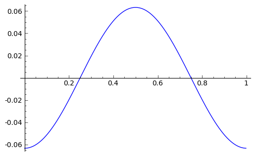
Rather encouraging.